ConCat/Split 3.1.4.1 serial key or number

Sketch

Copyright © 2005 to 2012 Eugene K. Ressler.

This manual is for , version 0.3 (build 7), Friday, February 24, 2012, a program that converts descriptions of simple three-dimensional scenes into line drawings. This version generates or code suitable for use with the TeX document processing system.

is free software. You can redistribute it and/or modify it under the terms of the GNU General Public License as published by the Free Software Foundation; either version 3, or (at your option) any later version.

Sketch is distributed in the hope that it will be useful, but WITHOUT ANY WARRANTY; without even the implied warranty of MERCHANTABILITY or FITNESS FOR A PARTICULAR PURPOSE. See the GNU General Public License for more details.

You should have received a copy of the GNU General Public License along with ; see the file COPYING.txt. If not, see .

--- The Detailed Node Listing ---

About sketch

Introduction by example

Swept objects

Input language

Basics

Literals

Arithmetic expressions

Options

Point lists

Drawables

• Dots: Draw dots.
• Lines: Draw polylines.
• Curves: Draw curves.
• Polygons: Draw polygons.
• Specials: Embed raw LaTeX and .
• Sweeps: Draw sweeps of dots and polylines.
• Blocks: Group other drawables.
• Repeats: Draw transformed copies of objects.
• Puts: Draw one object transformed.

Sweeps

Definitions

Global environment

• Global options: Attributes of the entire drawing.
• Camera: A final camera transformation of the scene.
• Picture box: Setting the bounding box and 2d clipping.
• Frame: Adding a box around the drawing.
• Language: Setting the output language.

Building a drawing

Caveats

Hidden surface removal and polygon splitting

1 About sketch

is a small, simple system for producing line drawings of two- or three-dimensional objects and scenes. It began as a way to make illustrations for a textbook after we could find no suitable tool for this purpose. Existing scene processors emphasized GUIs and/or photo-realism, both un-useful to us. We wanted to produce finely wrought, mathematically-based illustrations with no extraneous detail.

accepts a tiny scene description language and generates or code for LaTeX. The language is similar to , making it easy to learn for current users. See for information on . is similar. See . One can easily include arbitrary or drawings and text over, in, or under drawings, providing access to the full power of LaTeX text and mathematics formatting in a three-dimensional setting.

1.1 Reporting bugs and recommending improvements.

The group is the best place to report bugs and make improvements. A second method that will probably produce a slower response is email to . We will try to respond, but can't promise. In any event, don't be offended if a reply is not forthcoming. We're just busy and will get to your suggestion eventually.

For bugs, attach a input file that causes the bad behavior. Embed comments that explain what to look for in the behavior of or its output.

A recommendation for improvement from one unknown person counts as one vote. We use overall vote tallies to decide what to do next as resources permit. We reserve the right to assign any number of votes to suggestions from people who have been helpful and supportive in the past.

1.2 Contributions

If you intend to implement an enhancement of your own, that's terrific! Consider collaborating with us first to see if we're already working on your idea or if we can use your work in the official release.

2 Introduction by example

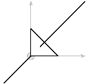
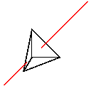
The input language will seem familiar to users of the package for LaTeX. The following program draws a triangular polygon pierced by a line.

polygon(0,0,1)(1,0,0)(0,1,0) line(-1,-1,-1)(2,2,2) The coordinate system is a standard right-handed Cartesian one.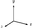

2.1 Hello world

The program above is nearly the simplest one possible, the equivalent of a “hello world” program you might find at the start of a programming language text. If it is saved in the file simple.sk, then the command

sketch simple.sk -o simple.tex creates a file simple.tex containing commands to draw these objects on paper. The contents of simple.tex look like this. \begin{pspicture}(-1,-1)(2,2) \pstVerb{1 setlinejoin} \psline(-1,-1)(.333,.333) \pspolygon[fillstyle=solid,fillcolor=white](0,0)(1,0)(0,1) \psline(.333,.333)(2,2) \end{pspicture} The hidden surface algorithm of has split the line into two pieces and ordered the three resulting objects so that the correct portion of the line is hidden.

If you've noticed that the projection we are using seems equivalent to erasing the z-coordinate of the three-dimensional input points, pat yourself on the back. You are correct. This is called a . The z-coordinate axis is pointing straight out of the paper at us, while the x- and y-axes point to the right and up as usual.

The resulting picture file can be included in a LaTeX document with . Alternately, adding the command line option -T¹causes the to be wrapped in a short but complete document, ready to run though LaTeX. In a finished, typeset document, the picture looks like this. (The axes have been added in light gray.)

It is important to know that only the “outside” of a polygon is normally drawn. The is where the vertices given in the command appear in counter-clockwiseorder. Thus, if the command above had been

polygon(0,1,0)(1,0,0)(0,0,1) the polygon would not appear in the picture at all. It would have been from the scene. This culling behavior may seem strange, but stay tuned.

2.2 Options

Many and options work just fine in . If generating , the code

polygon[fillcolor=lightgray,linewidth=3pt](0,0,1)(1,0,0)(0,1,0) line[linestyle=dotted](-1,-1,-1)(2,2,2) produces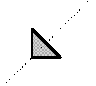

To produce , the corresponding code is

polygon[fill=lightgray,line width=3pt](0,0,1)(1,0,0)(0,1,0) line[style=dotted](-1,-1,-1)(2,2,2) global { language tikz } The final instructs to produce code as output rather than the default, . Note that fill color and style options both conform to syntax rules. The resulting output is \begin{tikzpicture}[join=round] \draw[dotted](-1,-1)--(.333,.333); \filldraw[fill=lightgray,line width=3pt](0,0)--(1,0)--(0,1)--cycle; \draw[dotted](.333,.333)--(2,2); \end{tikzpicture} The remaining examples of this manual are in PSTricks style.

2.3 Drawing a solid

Let's try something more exciting. has no notion of a solid, but polygonal can be used to represent the boundary of a solid. To the previous example, let's add three more triangular polygons to make the faces of an irregular tetrahedron.

% vertices of the tetrahedron def p1 (0,0,1) def p2 (1,0,0) def p3 (0,1,0) def p4 (-.3,-.5,-.8) % faces of the tetrahedron. polygon(p1)(p2)(p3) % original front polygon polygon(p1)(p4)(p2) % bottom polygon(p1)(p3)(p4) % left polygon(p3)(p2)(p4) % rear % line to pierce the tetrahedron line[linecolor=red](-1,-1,-1)(2,2,2) This example uses , which begin with . These or give names to points, which are then available as by enclosing the names in parentheses, e.g. . The parentheses denote that the names refer to points; they are required. There can be no white space between them and the name.

As you can see, comments start with as in TeX and extend to the end of the line (though will work as well). White space, including spaces, tabs and blank lines, has no effect in the language.

If we look inside the TeX file produced by , there will be only three polygons. The fourth has been culled because it is a “back face” of the tetrahedron, invisible to our view. It is unnecessary, and so it is removed.

In some drawings, polygons act as zero-thickness solid surfaces with both sides visible rather than as the faces of solid objects, where back faces can be culled. For zero-thickness solids, culling is a problem. One solution is to use a pair of polygons for each zero-thickness face, identical except with opposite vertex orders. This is unwieldy and expensive. A better way is to set the internal option to in the usual manner.

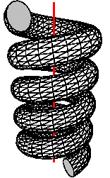
polygon[cull=false](p1)(p2)(p3) The following shows the same helix shape drawn first with (the default) and then .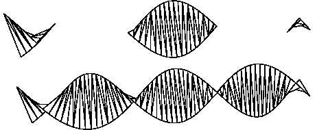

We'll soon see how to produce these helixes with a few lines of language code.

It may be tempting to turn culling off gratuitously so that vertex order can be ignored. This is not a good idea because output file size and TeX and Postscript processing time both depend on the number of output polygons. Culling usually improves performance by a factor of two. On the other hand, globally setting is reasonable while debugging. See Global options and Limits on error detection.

2.4 Special objects

We can add labels to a drawing by using objects, which provide a way to embed raw LaTeX and code. Adding this to the tetrahedron does the trick.

special |\footnotesize \uput{2pt}[ur]#1{$P1$} \uput[r]#2{$P2$} \uput[u]#3{$P3$} \uput[d]#4{$P4$}| (p1)(p2)(p3)(p4) Here is the result.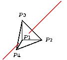

There are several details to note here. First, the quoting convention for the raw code is similar to the LaTeX command. The first non-white space character following is understood to be the quote character, in this case |. The raw text continues until this character recurs.

Second, the argument references , , , and refer to point, vector, or scalar values in the list that follow. This is similar to TeX macro syntax. The transformed and two-dimensional projections of these three-dimensional points are substituted in the final output. An argument reference of the form is replaced with the angle in degrees of the two-dimensional vector that connects the projections of the two respective argument points, here and . The substituted angle is enclosed in curly braces . When output is being generated, the angle is rounded to the nearest degree because non-integer angles are not allowed by primitives.

As of Version 0.3 of , special arguments may be scalars or vectors in addition to points. References to scalar arguments are merely replaced with a number formatted just as any point coordinate. References to vectors become two-dimensional points. The tick operator that selects individual components of points and vectors elsewhere in (see for example Affine arithmetic) can also be applied to point and vector argument references. All three dimensions of a transformed point or vector can also be substitued with . See Specials for details.

By default, objects are printed last, overlaying all other objects in the scene. If you specify the internal option , the hidden surface algorithm considers the entire special object to be the first point () in the argument list. If that point is behind (of smaller z-component than) any drawable, then the entire special object is drawn before that drawable, so the drawable obscures parts of the special object that overlaps it. In our example, is the front-most point in the scene (has the largest z-component), so adding has no effect.

With option , a special is drawn before, hence appears under any of the objects handled by the hidden surface algorithm. This is how the light gray axes were added to the “hello world” example Hello world.

objects are powerful, with many possible uses.

2.5 Transforms

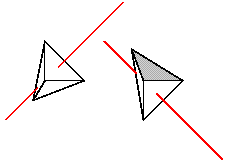
Now let's add a second copy of the pierced tetrahedron. We'll rotate the copy 90 degrees about the x-axis with the origin as so we can see the back, then translate it to the right—in the positive x-direction—so it doesn't collide with the original. To help us see what's going on, make the back side gray.

def pierced_tetrahedron { def p1 (0,0,1) def p2 (1,0,0) def p3 (0,1,0) def p4 (-.3,-.5,-.8) polygon(p1)(p2)(p3) % original polygon(p1)(p4)(p2) % bottom polygon(p1)(p3)(p4) % left polygon[fillcolor=lightgray](p3)(p2)(p4) % rear line[linecolor=red](-1,-1,-1)(2,2,2) } {pierced_tetrahedron} % tetrahedron in original position put { rotate(90, (0,0,0), [1,0,0]) % copy in new position then translate([2.5,0,0]) } {pierced_tetrahedron} Here the entire code of the previous example has been wrapped in a definition by forming a with braces (a single item would not need them). The point definitions nested inside the braces are . Their meaning extends only to the end of the block. The outer is called a definition because it describes something that can be drawn.

A drawable definition by itself causes nothing to happen until its name is referenced. Drawable references must be enclosed in curly braces, e.g. , with no intervening white space. In the code above, the first reference is a plain one. Its effect is merely to duplicate the earlier drawing. Almost any series of commands may be replaced with without changing its meaning.

The command supplies a second reference, this time with a applied first. The transform turns the tetrahedron 90 degrees about the origin. The axis of rotation is the vector [1,0,0]. By the , this causes the top of the tetrahedron to rotate toward the viewer and the bottom away. The rule receives its name from the following definition:

Right hand rule. If the right hand is wrapped around any axis with the thumb pointing in the axis direction, then the fingers curl in the direction of positive rotation about that axis.

The transform moves the pyramid laterally to the right by adding the vector [2.5,0,0] to each vertex coordinate. The result is shown here.

2.6 Repeated objects

To draw seven instances of the tetrahedron, each differing from the last by the same transform, replace the last two commands of the previous example with

repeat { 7, rotate(15, (0,0,0), [1,0,0]) % copy in new position then translate([2,0,0]) } {pierced_tetrahedron} And the result....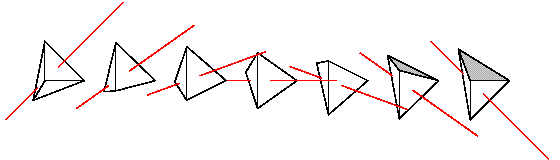

2.7 Swept objects

Many familiar shapes can be generated by sweeping simpler ones through space and considering the resulting path, surface, or volume. implements this idea in the command.

def n_segs 8 sweep { n_segs, rotate(180 / n_segs, (0,0,0), [0,0,1]) } (1,0,0) This code sweeps the point (1,0,0) eight times by rotating it 180/8 = 22.5 degrees each time and connecting the resulting points with line segments. The used here is a definition. References to scalars have no enclosing brackets at all.

2.7.1 Point sweeps

Sweeping a point makes a one-dimensional path, which is a polyline. Since we have swept with a rotation, the result is a circular arc. Here is what it looks like.

This is the first example we have seen of arithmetic. The expression causes the eight rotations to add to 180. If you're paying attention, you'll have already noted that there are nine points, producing eight line segments.

You can cause the swept point to generate a single polygon rather than a polyline by using the after the number of swept objects. Code and result follow

def n_segs 8 sweep { n_segs<>, rotate(180 / n_segs, (0,0,0), [0,0,1]) } (1,0,0)

2.7.2 Polyline sweeps

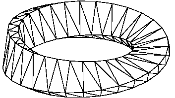
Sweeping a polyline produces a surface composed of many faces. The unbroken helix in the example Helix with cull set false then true is produced by this code (plus a surrounding rotation to make an interesting view; this has been omitted).

def K [0,0,1] sweep[cull=false] { 60, rotate(10, (0,0,0), [K]) then translate(1/6 * [K]) } line[linewidth=2pt](-1,0)(1,0) Again, 60 segments of the helix are produced by connecting 61 instances of the swept line. Options applied to the sweep, here , are treated as options for the generated polygon or polyline. Options of the swept line itself, here , are ignored, though with a warning. This is a definition, which must be referenced with square brackets, e.g. .

2.7.3 Nested sweeps

When the center point of rotation is omitted, the origin is assumed. When a point has only two coordinates, they are taken as x and y, with z=0 assumed. A toroid is therefore obtained with this code.

def n_toroid_segs 20 def n_circle_segs 16 def r_minor 1 def r_major 1.5 sweep { n_toroid_segs, rotate(360 / n_toroid_segs, [0,1,0]) } sweep { n_circle_segs, rotate(360 / n_circle_segs, (r_major,0,0)) } (r_major + r_minor, 0) For intuition, the idea of the code is to sketch a circle to the right of the origin in the xy-plane, then rotate that circle “out of the plane” about the y-axis to make the final figure. This produces the following. (A view rotation and some axes have been added.)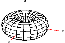

This example also shows that the swept object may itself be another . In fact, it may be any expression that results in a list of one or more points or, alternately, a list of one or more polylines and polygons. The latter kind of list can be created with a -enclosed block, perhaps following a or .

2.7.4 Polygon sweeps

Sweeping a polygon creates a closed surface with polygons at the ends, which are just copies of the original, appropriately positioned. See Solid coil example. Options on the swept polygon, if they exist, are applied to the ends. Otherwise the sweep options are used throughout.

2.7.5 Polyline sweeps with closure

A polyline sweep with a closure tag creates another kind of closed surface. First, the polyline segments are connected by faces, just as without the closure tag. Then, each set of end points is joined to make a polygon, one for each end. A code for several views of a cylindrical prism follows.

def n_cyl_segs 20 def n_views 5 def I [1,0,0] def endopts [fillcolor=lightgray] repeat { n_views, rotate(180/n_views, [I]) then translate([I] * 2.1) } sweep[endopts]{ n_cyl_segs<>, rotate(360/n_cyl_segs, [0,1,0]) } line[fillcolor=white](1,-1)(1,1) It produces this drawing.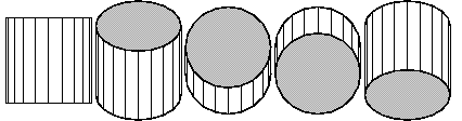

The options of the swept line, if any, are applied to the faces produced by sweeping the line, but not the end polygons. Otherwise, the sweep options are applied throughout. The in this example is an definition. References to options must be enclosed in square brackets, e.g.  . You can concatenate several sets of options with a single reference, e.g.  would cause the option definitions for , , and to appear in sequence in the output created by the command containing the reference. Happily, the syntax of is such that options references can never be confused with vector references. While not apparent in this example, options references are useful when defining many objects with a similar appearance.

2.7.6 Affine arithmetic

The arithmetic above hints at a larger truth. operators work on scalars, vectors, points, and transforms according to the general rules of . This can be helpful for setting up diagrams with computed geometry. For example, if you have triangle vertices through and need to draw a unit normal vector pointing out of the center of the triangle, this code does the trick.

def p1 (1,0,0) def p2 (0,0.5,0) def p3 (-0.5,-1,2) def O (0,0,0) def N unit( ((p3) - (p2)) * ((p1) - (p2)) ) def n1 ((p1)-(O) + (p2)-(O) + (p3)-(O)) / 3 + (O) def n2 (n1)+1655 polygon(p1)(p2)(p3) line[arrows=*->](n1)(n2) The first line computes the cross product of two edge vectors of the triangle and scales it to unit length. The second computes the average of the vertices. Note that subtraction and addition of the origin effectively convert vectors to points and vice versa. The line command draws the normal at the correct spot.

Two caveats regarding this example remain. First, the only way to use -style arrows is with . The alternative syntax for arrows is not allowed in . Second, you might like to eliminate the third and write instead the following.

line[arrows=*->](n1) (n1)+1655 This is not allowed. The point lists in drawables may consist only of explicit points or point references. You may, however, use arithmetic to calculate point components. The following works, though it's a little cumbersome. line[arrows=*->](n1)((n1)'x+(N)'x, (n1)'y+(N)'y, (n1)'z+(N)'z) Obviously, the 'x extracts components of points and vectors.

2.7.7 More to learn

This is not the end of the story on sweeps! We invite the reader into the main body of this documentation Sweeps to learn more.

Who knows where you'll finish?

3 Input language

This chapter describes the input language in detail.

3.1 Basics

input is plain ASCII text, usually stored in an input file. It describes a , so the sketch language is a . input is also . It merely declares what the scene ought to look like when drawing is complete and says very little about how should do its work. commands are not executed sequentially as in the usual programming language. They merely contribute to that declaration.

A few syntactic details are important. Case is significant in the language. With a few exceptions, white space is not. This includes line breaks. Comments begin with or and extend to the end of the line. You can disable a chunk of syntactically correct code by enclosing it in a . There is a simple “include file” mechanism. The command

input{otherfile.sk} causes the contents of otherfile.sk to be inserted as though they were part of the current file.

3.1.1 Identifiers

Identifiers in are references to earlier-defined options, scalars, points, vectors, transforms, drawables, and tags. Definitions are explained in Definitions.

An identifier consists of a leading letter followed by letters, numbers and underscores. The last character may not be an underscore. Keywords cannot be used as identifiers, and reserved words ought to be avoided. See Key and reserved words.

3.1.2 Key and reserved words

The keywords of are and . The parser will note a syntax error if any of these are used in place of a proper identifier.

In addition, there are reserved words that can currently be defined by the user, but with the risk that future versions of will reject those definitions. The reserved words are and .

3.1.3 Literals

Literals in include scalars, points, vectors, and transforms. Literals, along with defined object references, are used in arithmetic expressions. See Arithmetic.

3.1.3.1 Scalar literals

Scalar literals are positive floating point numbers with syntax according to C conventions. The following are some examples.

0 1004 .001 8.3143 3. 1.60E-19 6.02e+23

Scalar literals may not contain embedded spaces.

3.1.3.2 Point and vector literals

Points and vector literals have these forms respectively.

(X,Y,Z) [X,Y,Z]

Each of the components is itself a scalar expression. The z-components are optional and default to zero.

3.1.3.3 Transform literals

Most transform literals are formed by . These are summarized in the following table.

Constructor	Param types	Description
	scalar,point,vector	Rotate degrees about point with axis according to the right hand rule. See Right hand rule. and are both optional and default to the origin and the z-axis respectively.
	vector	Translate by .
	scalar	Scale uniformly by factor .
	vector	Scale along each axis by components of .
	—	Same as .
	scalar	Perspective projection with view center at origin and projection plane z=-.
	scalar	Perspective transform identical to except that the z-coordinate of the transformed result is , usable by the hidden surface algorithm.
	point,vector,vector	View transform similar to that of 's. The eye point is translated to the origin while a rotation is also applied that makes the view direction vector and the view “up” vector point in the negative z- and the y-directions respectively. If is omitted, it defaults to [0,1,0]. When is omitted, may be also; it defaults to , a vector pointing from the eye toward the origin.
	point,point,vector	An alternate form of above where the view direction parameter is replaced with a “look at” point , i.e., a point where the viewer is focusing her attention. This form of view is equivalent to , where is a direction vector. is optional and defaults to [0,1,0].
	16 scalars	Direct transform matrix definition. Each of the a_ij is a scalar expression. See text for details.

The constructor is not generally useful because it defeats hidden surface removal by collapsing the scene onto a single plane. It is a special purpose transform for drawing pictures of scenes where three-dimensional objects are being projected onto planes. See, for example, Overview.

The direct transform constructor allows direct entry of a 4x4 transformation matrix. Most 3d graphics systems, including , use 4-dimensional homogeneous coordinates internally. These are transformed by multiplication with 4x4 matrices. The built-in constructors (, , etc.) are all translated internally to such 4x4 matrices. For more information on homogeneous coordinate transformations, see any good computer graphics textbook. The direct transform feature of allows you to enter a matrix of your own choice. There are not many cases where this is useful, but if you do need it, you need it badly!

3.1.4 Arithmetic expressions

Arithmetic expressions over literals and defined identifiers are summarized in the following tables.

3.1.4.1 Two-operand (binary) forms and precedence

Most two-operand binary forms have meanings dependent on the types of their arguments. An exhaustive summary of the possibilities is given in the following table.

Left	Op	Right	Result	Description
scalar	scalar	scalar	Scalar sum.
vector	vector	vector	Vector sum.
point	vector	point	Point-vector affine sum.
vector	point	"	"
scalar	scalar	scalar	Scalar difference.
vector	vector	vector	Vector difference.
point	point	vector	Point-point affine difference.
point	vector	point	Point-vector affine difference.
scalar	or	scalar	scalar	Scalar product.
scalar	or	vector	vector	Scalar-vector product.
vector	or	scalar	"	"
vector	vector	vector	Vector cross-product.
vector	vector	scalar	Vector dot product.
scalar	scalar	scalar	Raise scalar to scalar power.
transform	integer	transform	Raise transform to integer power.
transform	or	point	point	Affine point transform (right-to-left).
transform	or	vector	vector	Affine vector transform (right-to-left).
transform	or	transform	transform	Transform composition (right-to-left).
point	transform	point	Affine point transform (left-to-right).
vector	transform	vector	Affine vector transform (left-to-right).
transform	transform	transform	Transform composition (left-to-right).
scalar	scalar	scalar	Scalar division.
vector	scalar	vector	Vector component-wise division by scalar.
point	, , or	scalar	Point component extraction.
vector	, , or	scalar	Vector component extraction.

Operator precedence is shown in this table.

Op	Precedence
highest (most tightly binding)
(unary negation)
lowest (least tightly binding)

All operations are left-associative except for ^. Parentheses ( )are used for grouping to override precedence in the usual way.

As you can see, the dot operator .is usually a synonym for run-of-the-mill multiplication, *. The meanings differ only for vector operands. The operator merely reverses the operand order with respect to normal multiplication *. The intent here is to make compositions read more naturally. The code

(1,2,3) then scale(2) then rotate(30) then translate([1,3,0])

expresses a series of successive modifications to the point, whereas the equivalent form

translate([1,3,0]) * rotate(30) * scale(2) * (1,2,3)

will be intuitive only to mathematicians (and perhaps Arabic language readers).

3.1.4.2 Unary forms

Unary or one-operand forms are summarized in the following table, where stands for the operand.

Op	Operand	Result	Description
scalar	scalar	Unary scalar negation.
vector	vector	Unary vector negation.
vector	scalar	Vector length.
vector	vector	Unit vector with same direction.
scalar	scalar	Scalar square root.
scalar	scalar	Trigonometric sine ( in degrees).
scalar	scalar	Trigonometric cosine ( in degrees).
scalar	scalar	Inverse sine ( in degrees).
scalar	scalar	Inverse cosine ( in degrees).
scalar	scalar	Polar angle in degrees of vector [X,Y].
transform	transform	Inverse transform.

Errors are reported when , , , , , , and fail due to operands outside their respective domains.

3.1.5 Options

Syntax:

[=,=,...]

Options are used to specify details of the appearance of drawables. As shown above, they are given as comma-separated key-value pairs.

3.1.5.1 options

When is selected (the default), permissible key-value pairs include all those for similar objects. For example, a polygon might have the options

[linewidth=1pt,linecolor=blue,fillcolor=cyan] merely passes these on to without checking or modification. Option lists are always optional. A missing options list is equivalent to an empty one [].

When a has options for both its face and its edges, and the polygon is split by the hidden surface algorithm, must copy the edge options to s for the edge segments and the face options to s. Options known to for purposes of this splitting operation include , , , , , , , , , , , and .

3.1.5.2 options

options are handled much as for . Though often allows colors and styles to be given without corresponding keys, for example,

\draw[red,ultra thick](0,0)--(1,1); this is not permitted in . To draw a red, ultra-thick line in , the form is line[draw=red,style=ultra thick](0,0)(1,1)

Just as for , when a has options for both its face and its edges, and the polygon is split by the hidden surface algorithm, must copy the edge options to s for the edge segments and the face options to s. options known to for purposes of this splitting operation include , , , , , , , , , , , , , , , , and .

The option can contain both face and edge information, so must check the style value. Values known to include , , , , , , , , , , , , , , , , , , , , and .

3.1.5.3 Dots in

does not have a command as does PSTricks. Instead, emits dots as circles. The diameter may be set using the option borrowed from PSTricks. The option will be removed from the option list in the output command. Other options work in the expected way. For example, sets fill color and sets line color of the circles.

3.1.5.4 user-defined styles

allows named styles defined by the user, for example

\tikzstyle{mypolygonstyle} = [fill=blue!20,fill opacity=0.8] \tikzstyle{mylinestyle} = [red!20,dashed] Since has no information on the contents of such styles, it omits them entirely from lines, polygons, and their edges during option splitting. For example, polygon[style=mypolygonstyle,style=thick](0,0,1)(1,0,0)(0,1,0) line[style=mylinestyle](-1,-1,-1)(2,2,2) produces the output \draw(-1,-1)--(.333,.333); \filldraw[thick,fill=white](0,0)--(1,0)--(0,1)--cycle; \draw(.333,.333)--(2,2); Note that the user-defined styles are not present. Sketch also issues warnings: warning, unknown polygon option style=mypolygonstyle will be ignored warning, unknown line option style=mylinestyle will be ignored

The remedy is to state explicitly whether a user-defined style should be attched to polygons or lines in the output using pseudo-options and ,

polygon[fill style=mypolygonstyle,style=thick](0,0,1)(1,0,0)(0,1,0) line[line style=mylinestyle](-1,-1,-1)(2,2,2) Now, the output is \draw[mylinestyle](-1,-1)--(.333,.333); \filldraw[mypolygonstyle,thick](0,0)--(1,0)--(0,1)--cycle; \draw[mylinestyle](.333,.333)--(2,2);

A useful technique is to include user-defined style definitions in code as s with option to ensure that the styles are emitted first in the output, before any uses of the style names. ² For example,

special|\tikzstyle{mypolygonstyle} = [fill=blue!20,fill opacity=0.8]|[lay=under] special|\tikzstyle{mylinestyle} = [red!20,dashed]|[lay=under] The author is responsible for using the key, or , that matches the content of the style definition.

3.1.5.5 Transparency

Both and support polygon options that have the effect of making the polygon appear transparent. For , keyword was used during initial development of transparency features, and was adopted later. honors both. uses only. When transparent polygons are in the foreground, objects behind them (drawn earlier) are visible with color subdued and tinted. The hidden surface algorithm of works well with such transparent polygons.

Note that must be used for rear-facing polygons to be visible when positioned behind other transparent surfaces.

3.1.5.6 Internal options

There are also internal options used only by and not passed on to . These are summarized in the following table.

Key	Possible values	Description
,	Turn culling of backfaces on and off respectively for this object. The default value is .
, ,	Force this object to be or all other objects in the depth sort order created by the hidden surface algorithm. The default value guarantees that output due to the will be visible.
,	Turn splitting of sweep-generated body polygons on and off respectively. See Sweeps. The default value causes “warped” polygons to be split into triangles, which avoids mistakes by the hidden surface algorithm.

3.1.6 Point lists

Syntax:

(,,)(,,)...

A sequence of one or more points makes a point list, a feature common to all drawables. Each of the point components is a scalar arithmetic expression. Any point may have the z-component omitted; it will default to z=0.

3.2 Drawables

Drawables are simply objects that might appear in the drawing. They include dots, polylines, curves, polygons, and more complex objects that are built up from simpler ones in various ways. Finally, objects are those composed of LaTeX or code, perhaps including coordinates and angles computed by .

• Dots: Draw dots.
• Lines: Draw polylines.
• Curves: Draw curves.
• Polygons: Draw polygons.
• Specials: Embed raw LaTeX and .
• Sweeps: Draw sweeps of dots and polylines.
• Blocks: Group other drawables.
• Repeats: Draw transformed copies of objects.
• Puts: Draw one object transformed.

3.2.1 Dots

Syntax:

dots[]

This command is the three-dimensional equivalent of the command .

3.2.2 Lines

Syntax:

line[]

This command is the three-dimensional equivalent of the command .

3.2.3 Curves

Syntax:

curve[]

This command is the three-dimensional equivalent of the command . It is not implemented in the current version of .

3.2.4 Polygons

Syntax:

polygon[]

This command is the three-dimensional equivalent of the command . The hidden surface algorithm assumes that polygons are convex and planar. In practice, drawings may well turn out correctly even if these assumptions are violated.

3.2.5 Specials

Syntax:

special $$[]

Here can be any character and is used to delimit the start and end of . The command embeds in the output after performing substitutions as follows.

• where is a positive integer is replaced by the 'th value in . Point and vector arguments become two-dimensional points, which are the transformed 3d arguments projected onto the - plane. This allows two-dimentional output elements such as labels to be easily positioned with respect to three-dimensional features in the drawing. Scalar arguments are subsituted directly. No transformation is applied.
• is also replaced as above.
• is replaced as above for points or vectors. It is an error for the 'th argument to be a scalar.
• , , or is replaced, respectively, by the scalar , , or -coordinate of the argument point or vector. It is an error for the 'th argument to be a scalar.
• is replaced by the three-dimensional transformed argument. Note that if a perspective transformation has been applied, the -coordinate has little geometric significance, though it accurately indicates relative depth.
• where and are positive integers is replaced by a string where is the polar angle of a vector from the 'th point in to the 'th point projected into the x-y plane. It is an error for the 'th or 'th argument to be a scalar or a vector.
• is also replaced as above.
• is replaced with .

The forms with braces { } are useful when the argument is immediately followed by a digit or a tick character that is part of the TeX code.

The only useful option of is , which determines if the substitued raw text is emitted before, after, or using the first point in as an indicator of depth. These occur, respectively, with , , and . See Special objects and TikZ/PGF user-defined styles for examples. See Internal options.

3.2.6 Sweeps

Syntax:

sweep { , , , ..., }[] sweep { <>, , , ...,

Often, we will have a set of 1-D arrays, and we would like to construct a 2D array with those vectors as either the rows or columns of the array. This may happen because we have data from different sources we want to combine, or because we organize the code with variables that are easy to read, and then want to combine the variables. Here are examples of doing that to get the vectors as the columns.

[[1 4] [2 5] [3 6]] [[1 4] [2 5] [3 6]]

Or rows:

[[1 2 3] [4 5 6]] [[1 2 3] [4 5 6]]

The opposite operation is to extract the rows or columns of a 2D array into smaller arrays. We might want to do that to extract a row or column from a calculation for further analysis, or plotting for example. There are splitting functions in numpy. They are somewhat confusing, so we examine some examples. The numpy.hsplit command splits an array "horizontally". The best way to think about it is that the "splits" move horizontally across the array. In other words, you draw a vertical split, move over horizontally, draw another vertical split, etc… You must specify the number of splits that you want, and the array must be evenly divisible by the number of splits.

[[1 2] [4 5]] [[3 5] [6 9]] [[1] [4]] [[2] [5]] [[3] [6]] [[5] [9]]

In the numpy.vsplit command the "splits" go "vertically" down the array. Note that the split commands return 2D arrays.

[[1 2 3 5]] [[4 5 6 9]] (1, 4)

An alternative approach is array unpacking. In this example, we unpack the array into two variables. The array unpacks by row.

[1 2 3 5] [4 5 6 9]

To get the columns, just transpose the array.

[1 4] [2 5] [3 6] [5 9] (2,)

Note that now, we have 1D arrays.

You can also access rows and columns by indexing. We index an array by [row, column]. To get a row, we specify the row number, and all the columns in that row like this [row, :]. Similarly, to get a column, we specify that we want all rows in that column like this: [:, column]. This approach is useful when you only want a few columns or rows.

[4 5 6 9] [4 5 6 9] [3 6] (2,)

Note that even when we specify a column, it is returned as a 1D array.